Continuous probability distribution

Last updated Nov 13, 2022

• Mathematics

A continuous probability distribution is the probability distribution of a continuous random variable. A common distribution is the normal distribution.

Generally, the probability of a continuous set of data can be found through the area under the graph. This applies to density functions that are rectangular, linear, or triangular in nature and more. Therefore, if a probability is asked for a specific singular value (e.g., $P(X = a)$), the answer will always be 0.

Also known as the normal curve or Gaussian distribution. Its curve follows the shape of a bell-shaped curve and it describes many sets of data that occur. The curve is symmetrical about a vertical axis through the mean $\mu$.

$\mu$ offsets the location of the bell-shaped curve horizontally; $\sigma$ offsets the height (proportional) and spread (inversely proportional) of the bell-shaped curve.

A normal distribution is only valid if three conditions are met:

• $f(X) > 0$ for all values of $x$. In other words, the graph must be above the x-axis.
• The total area under the curve must be equal to 1.
• The normal curve must be symmetric about the vertical axis at $x = \mu$. This means that the area to the left or right of $\mu$ are both $\frac 1 2$.

The notation to describe a normal distribution is: $$ X \sim N(\mu, \sigma^2) $$

There are certain values that are good to know when it comes to the area bound between standard deviations.

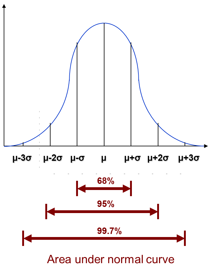
• $P(\mu - \sigma < X < \mu + \sigma) = 0.68$
• $P(\mu - 2\sigma < X < \mu + 2\sigma) = 0.95$
• $P(\mu - 3\sigma < X < \mu + 3\sigma) = 0.997$

To compute the area for different normal curves with different $\mu$ and $\sigma$ values, standardisation needs to be done. This standard form is known as standard normal distribution. A standard normal distribution has the following notation: $$ Z \sim N(0, 1) $$ Standard normal distribution standardises the different normal curves into one with a mean of 0 and a standard deviation of 1.

Once standardised, any normal distribution can be used together with the standard normal Z-table to compute the area under all different curves.

In order to standardise a random variable $X$ into its standardised value $Z$, the following formula needs to be done: $$ Z = \frac {X - \mu} \sigma $$ In order to read the standard normal Z-table, the value of $z$ must be a positive value.

Using the standard normal Z-table, we can find $\phi (z)$. It is important to note the following: $$ \phi (z) = P(Z \leq z) $$

# Normal approximation to discrete probability distributions

Since normal distribution is a form of continuous probabiity distribution, while it is possible to approximate it to a discrete probability distribution, continuity correction must be done to convert the discrete random variable into one of continuous nature.

Generally, to perform continuity correction, each discrete number must be treated as a continuous interval between a $\pm$ 0.5 value.

Example Provided $X = 1$, correction will be done such that $X$ becomes a range ($0.5 < X < 1.5$).

# Normal approximation from binomial distribution

When a binomial distribution has a high number of independent trails ($n$) and a low probability ($p$), we can approximate the binomial distribution into a normal distribution.

Expressed mathematically, when $n \to \infty, \space p \approx 0.5$ such that $np > 5, nq > 5$, $$ X \sim B(n, p) \approx X \sim N (np, npq) $$

# Normal approximation from Poisson distribution

When a Poisson distribution has an average value ($\lambda$) sufficiently larger than its square root ($\sqrt \lambda$), we can approximate the Poisson distribution into a normal distribution.

Expressed mathematically, when $\lambda > 10$: $$ X \sim P_O (\lambda) \approx X \sim N (\lambda, \lambda) $$

# Normal approximation to sampling distribution of the sample mean

If $X_1, X_2, …, X_n$ is a random sample (of size $n$) taken from a population where $X \sim N (\mu, \sigma^2)$, then the sample mean ($\bar X$) follows a normal distribution.

Expressed mathematically, when $X \sim N (\mu, \sigma^2)$, $$ \bar X \sim N(\mu, \frac {\sigma^2} n) $$

The Theorem states that if $X_1, X_2, …, X_n$ is a random sample of a large size $n$ (where $n \geq 30$) and $X$ is of any distribution with mean $\mu$ and variance $\sigma^2$, the sample mean ($\bar X$) is approximately normal.

Expressed mathematically, when $n \geq 30$ and $\mu$ and $\sigma^2$ are present, $$ \bar X \sim N(\mu, \frac {\sigma^2} n) $$

A $t$-distribution is a type of normal distribution used for sample sizes that are small (where $n < 30$). It looks similar to a normal $z$-distribution, but differs slightly. As the $df$ of a $t$-distribute increases, the closer it gets to being a $z$-distribution.

$t$-distributions are varied in shape through the degree of freedom $df$ they have. The degree of freedom is equal to the difference of one from the sample size. Expressed mathematically: $$ df = n - 1 $$

In order to find the value in a $t$-distribution, the following formula needs to be done: $$ t = \frac {\bar X - \mu} {\frac s {\sqrt n}} $$ where:

• $\bar X$ is the sample mean;
• $\mu$ is the population mean;
• $s$ is the sample standard deviation; and
• $n$ is the sample size.

The $t$-distribution is not dependent on the population variance; therefore, it may be used in place of the $z$-distribution where:

• the population variance is unknown; or
• the sample size is small ($n < 30$).