Hypothesis testing

Last updated Jan 24, 2023

• Mathematics

Refers to the process involved in accepting or rejecting statements about a population’s parameters. These parameters usually are the mean ($\mu$) or a proportion ($p$).

In hypothesis testing, there are two hypotheses that are formulated in a particular test:

• The null hypothesis ($H_0$) is the statement about the parameter formulated for the purpose of testing whether it is to be accepted or rejected.
• The alternative hypothesis ($H_1$) is the statement that is accepted should the null hypothesis be rejected.

In a hypothesis test, there are two possible errors that can occur:

• A Type I error rejects the null hypothesis when it is true (i.e., false negative).
• A Type II error accepts the null hypothesis when it is false (i.e., false positive).

The probability of committing a Type I error is denoted by $\alpha$, and that of committing a Type II error is denoted by $\beta$.

In hypothesis testing, we only accept a hypothesis if there is no sufficient evidence for us to reject it. Therefore, when a hypothesis is accepted, it does not mean that we believe it is 100% true. We are hence more concerned about Type I errors than Type II errors.

1. Formulate the null hypothesis $H_0$ and the alternative hypothesis $H_1$ in statistical terms.
2. Decide whether to use a one-tailed or two-tailed test.
3. Set a level of significance $\alpha$.
4. Find the critical values and determine the rejection region $R$ from the critical values.
5. Select an appropriate test statistic and calculate the value of the test statistic.
6. Make the decision; if the test statistic falls in $R$, reject $H_0$, else accept $H_0$.

Where a null hypothesis exists such that $H_0 : \mu = \mu_0$, there are three possible alternative hypotheses $H_1$:

• $H_1 : \mu \neq \mu$;
• $H_1 : \mu \gt \mu$; or
• $H_1 : \mu \lt \mu$.

Where a null hypothesis exists such that $H_0 : \mu = \mu_0$, if the alternative hypothesis $H_1$ is:

• $H_1 : \mu \neq \mu$, then the test is two-tailed;
• $H_1 : \mu \gt \mu$ then the test is one-tailed; or
• $H_1 : \mu \lt \mu$, then the test is one-tailed.

The level of significance is usually denoted by $\alpha$%. The level of significance is also the probability of wrongly rejecting $H_0$ when $H_0$ is true (i.e., a false negative or a Type I error). Commonly-used values of the significance levels are 1%, 5%, and 10%.

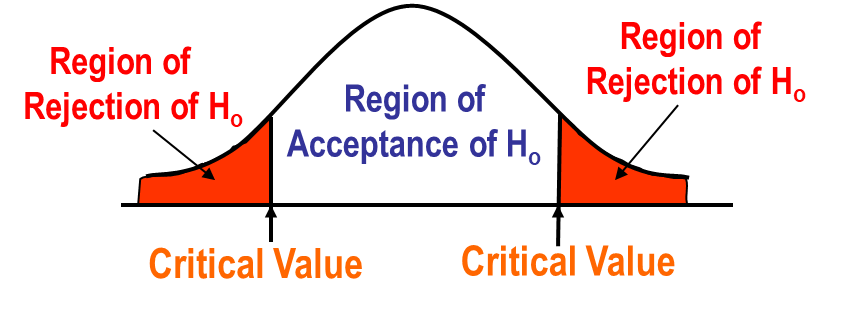
The critical value is the value arrived based on the level of significance decided. It divides the region of rejection and region of acceptance.

In a two-tailed test, the rejection region refers to the values below the negative and above the significance level.

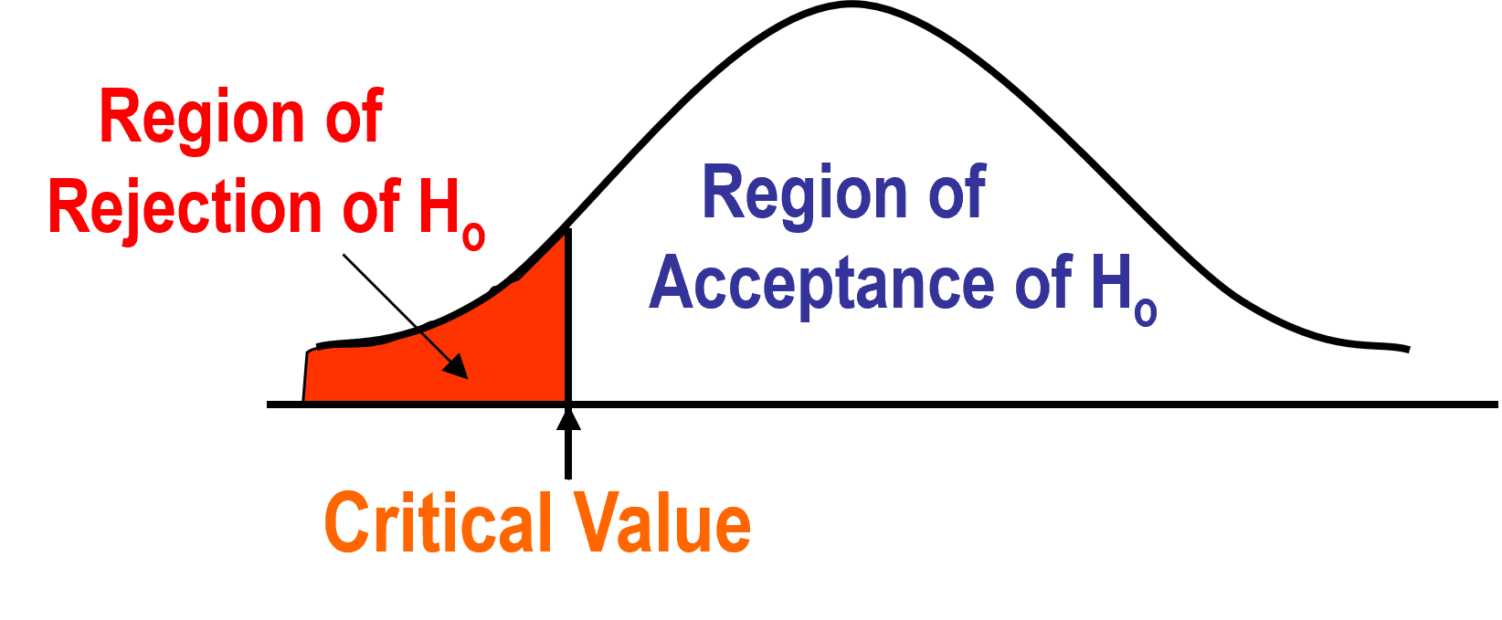
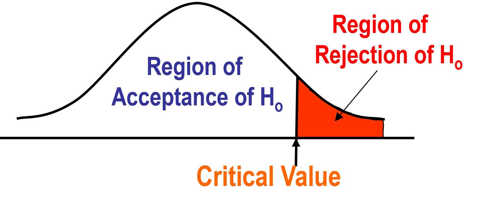
In a one-tailed test where $H_1: \mu < \mu_0$, the rejection region is the values below the negative of the significance level. In a one-tailed test where $H_1 : \mu > \mu_0$, the rejection region is the values above the significance level.

The critical values can be determined based on the significance level. Depending on whether the sample size is large ($n \geq 30$) or small ($n < 30$), we can refer to the $z$-distribution and $t$-distribution table respectively.

The test statistic is a value computed from the sample data used to decide whether to accept or reject the null hypothesis. The formula for calculating the test statistic is as such: $$ z = \frac {\bar X - \mu} {\frac \sigma {\sqrt n}} $$

If the population’s standard deviation $\sigma$ is unknown, it can be estimated with the sample standard deviation $\hat \sigma = s$: $$ z = \frac {\bar X - \mu} {\frac s {\sqrt n}} $$

Depending on whether the test static falls in the rejection or acceptance region, difference statements can be said.

When the test statistic falls in the rejection region, the test is said to be statistically significant and means that there is a significant difference between the sample statistic and the hypothesised population parameter.

A conclusion can therefore be made, stating such:

Since the test statistic $z$ falls in the rejection region, there is sufficient evidence at the $\alpha$% significance level to reject $H_0$. Therefore, we can accept $H_1$.

When the test statistic falls in the acceptance region, there is insufficient evidence to reject $H_0$, meaning that the test is statistically non-significant.

A conclusion can therefore be made, stating such:

Since the test statistic $z$ does not fall in the rejection region there is no sufficient evidence at the $\alpha$% significance level to reject $H_0$. Therefore we accept $H_0$.

The $p$-value is the probability of getting a test statistic value as extreme as the value actually obtained minimally. If the $p$-value is smaller than the significance level, the null hypothesis is rejected; otherwise, it is accepted.

The $p$-value is the probability of the rejection region. Therefore, to obtain the $p$-value:

If $H_1 : \mu \neq \mu_0$, $$ p = 2 \times (1 - \phi(z)) $$

If $H_1: \mu < \mu_0$ or $H_1 : \mu > \mu_0$, $$ p = 1 - \phi(z) $$